


Interpreting Isolation Forest’s predictions — and not only
 on [Unsplash](https://unsplash.com?utm_source=medium&utm_medium=referral)](https://cdn-images-1.medium.com/max/11520/0*fw1naEWsmO25wKq5)
The problem: how to interpret Isolation Forest’s predictions
More specifically, how to tell which features are contributing more to the predictions. Since Isolation Forest is not a typical Decision Tree (see Isolation Forest characteristics here), after some research, I ended up with three possible solutions:
1) Train on the same dataset another similar algorithm that has feature importance implemented and is more easily interpretable, like Random Forest.
2) Reconstruct the trees as a graph for example. The most important features should be the ones on the shortest paths of the trees. This is because of how Isolation Forest works: the anomalies are few and distinct, so it should be easier to single them out — in fewer steps, thus, shortest paths.
3) Estimate the Shapley values: the marginal feature contribution, which is a more standard way of identifying feature importance ranking.
Options 1 and 2 were not deemed as the best solutions to the problem, mainly because of the difficulties in how to pick a good algorithm — Random Forest, for example, operates differently than Isolation Forest, so it wouldn’t be very wise to use its feature importance output. Additionally, option 2 does not generalize and it would be like trying to do the algorithm’s work all over again.
For option 3, while there are a few libraries, like shap and shparkley, I had many issues using them with spark IForest, regarding both usability and performance.
The solution was to implement Shapley values’ estimation using Pyspark, based on the Shapley calculation algorithm described below.
The implementation takes a trained pyspark model, the spark dataframe with the features, the row to examine, the feature names, the features column name and the column name to examine, e.g. prediction. The output is the ranking of features, from the most to the least helpful.
What are the Shapley values?
The Shapley value provides a principled way to explain the predictions of nonlinear models common in the field of machine learning. By interpreting a model trained on a set of features as a value function on a coalition of players, Shapley values provide a natural way to compute which features contribute to a prediction.[14] This unifies several other methods including Locally Interpretable Model-Agnostic Explanations (LIME),[15] DeepLIFT,[16] and Layer-Wise Relevance Propagation.[17]
source: https://en.wikipedia.org/wiki/Shapley_value#In_machine_learning
Or as the python shap package states:
A game theoretic approach to explain the output of any machine learning model.
In other words, it is the average of the marginal contributions across all feature permutations. The following article has a good way of explaining what the marginal contribution is: Explain Your Model with the SHAP Values Use the SHAP Values to Explain Any Complex ML Modeltowardsdatascience.com
You can find the relevant code here.
From the article below with an example from game theory: “finding each player’s marginal contribution, averaged over every possible sequence in which the players could have been added to the group”. Thus, finding each feature’s marginal contribution, averaged over every possible sequence in which the features could have been selected. I’ll provide an algorithm and a visual example shortly :) One Feature Attribution Method to (Supposedly) Rule Them All: Shapley Values Among the papers that caught my eye at NIPS was this one, that made the lofty claim to have discovered a framework…towardsdatascience.com
Estimating Shapley Values with Pyspark
An approximation with Monte-Carlo sampling
First, select an instance of interest x, a feature j and the number of iterations M.
For each iteration, a random instance z is selected from the data and a random order of the features is generated.
Two new instances are created by combining values from the instance of interest x and the sample z.
The instance x+j is the instance of interest, but all values in the order before feature j are replaced by feature values from the sample z.
The instance x−j is the same as x+j, but in addition has feature j replaced by the value for feature j from the sample z.
The difference in the prediction from the black box is computed
](https://cdn-images-1.medium.com/max/2000/1*z53_nkTmNaJR-n-BwF8J9A.png)
All these differences are averaged and result in:
](https://cdn-images-1.medium.com/max/2000/1*Scpd6ZubMsdUuOwEX1HPrA.png) source
5.9 Shapley Values | Interpretable Machine Learning
A prediction can be explained by assuming that each feature value of the instance is a "player" in a game where the…christophm.github.io
source
5.9 Shapley Values | Interpretable Machine Learning
A prediction can be explained by assuming that each feature value of the instance is a "player" in a game where the…christophm.github.io
The advantages of using Shapley values:
“The difference between the prediction and the average prediction is fairly distributed among the feature values of the instance. […] In situations where the law requires explainability — like EU’s “right to explanations” — the Shapley value might be the only legally compliant method, because it is based on a solid theory and distributes the effects fairly.” . This is a very important advantage I believe.
You can use a sample of the dataset to compare the Shapley values.
The Shapley value is the only explanation method with a solid theory
The disadvantages of using Shapley values:
As one can imagine, the calculation of Shapley values requires a lot of computing time. Decreasing the number of iterations (M) reduces computation time, but increases the variance of the Shapley value. It makes sense that the iterations number should be large enough to accurately estimate the values, but small enough to complete the computation in a reasonable time. This is one of the main reasons for a scalable solution.
This article won’t focus on the ways to choose the right M, but it will provide a possible solution to use the whole dataset, or the greater part of it, for the calculation in a relatively reasonable time.
You need both the model and the data (feature vectors) to calculate them.
It can be misinterpreted. This is one issue I struggled with myself. “The Shapley value of a feature value is not the difference of the predicted value after removing the feature from the model training.” Instead, one should view the values as the contribution of a feature value to the difference between the actual prediction and the mean prediction.
It is not suitable for sparse solutions —meaning sparse vectors with few features within a sample. All the features are needed.
Using Pyspark
First of all, why Pyspark?
Because of the following statement:
“… the iterations number should be large enough to accurately estimate the values, but small enough to complete the computation in a reasonable time … “
Estimating Shapley Values requires a lot of computing time and if you are using Spark models, there’s a good chance your dataset ranges from big-ish to huge. So, it only makes sense to use Spark to help spread the computation to different workers and make things as efficient as possible. I mean, sure we’ll be using a udf for some part of the calculation, but even so, this will run on different workers, so in parallel.
It only makes sense to use Spark to help spread the computation to different workers and make things as efficient as possible
Ok then, how?
To calculate the Shapley values for all features following the algorithm description above using pyspark, the algorithm below was used:
Let’s start with a dataframe that has an ID column and features F1, F2, F3, F4.
The ID doesn’t have to be sequential but it has to be unique and can be generated with the ways described here. The reason for the ID column is because we need a row of interest so we need to identify this somehow within the dataset. We can also use a is_selected column (as you’ll notice in the code), but let’s go on with the explanation of the basic algorithm first.
The features can reside in one column e.g. features or in separate, it doesn’t really matter. In our example, let’s have them separate so that it is easier to see the values.
So, M consists of all the rows, each of the row is a z , so we have z1, z2 ... zM and let’s randomly choose zM-3, the fourth row from the end to be our row of interest x.
Note: x is filtered out as it doesn’t make sense to calculate xj for it
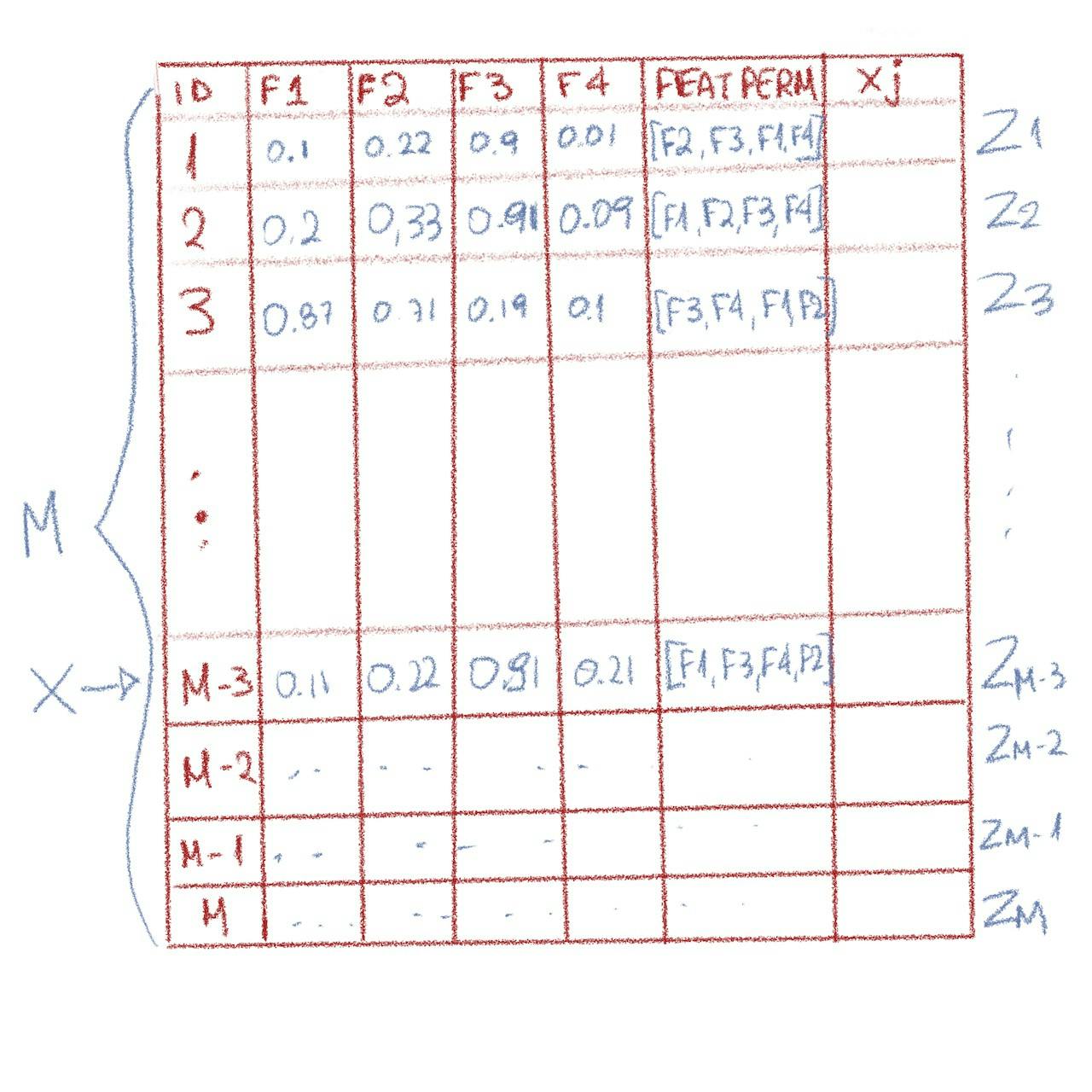 Example of the initial dataframe with a feature permutations column (created by Author)
Since we are going through all M rows, we need a feature permutation for each. The following function does exactly that. Given an array of feature names, and a dataframe df, it creates a column features_permutation with a feature permutation (list of features in some order) for each row.
import pyspark
from pyspark.sql import functions as F


def get_features_permutations(
        df: pyspark.DataFrame,
        feature_names: list,
        output_col='features_permutations'
):
    """
    Creates a column for the ordered features and then shuffles it.
    The result is a dataframe with a column `output_col` that contains:
    [feat2, feat4, feat3, feat1],
    [feat3, feat4, feat2, feat1],
    [feat1, feat2, feat4, feat3],
    ...
    """
    return df.withColumn(
        output_col,
        F.shuffle(
            F.array(*[F.lit(f) for f in feature_names])
        )
    )
Once we get the permutations we can start iterating the features to calculate x+j and x-j . Because we’ll be using a udf for this, we’ll be calculating both in one udf under one column xj for performance reasons (udfs can be expensive in pyspark).
Let’s start with j = F1.
The udf needs the name of the selected feature, feature j, the values of z1, and the feature permutation that corresponds to z1 . It also needs the ordered feature names and the row of interest values, x. The last two can be broadcasted.
So, for the following z1, x, feature permutation [F2, F3, F1, F4], the xj for j=F1 is calculated as seen below:
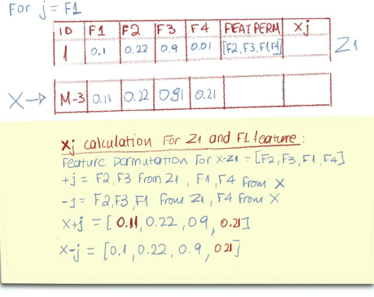 How xj (x-j and x+j) is calculated (source: Author)
The udf, as seen below, practically iterates the current feature permutation from where j=F1 is, so [F2, F3, F1, F4] in our example becomes [F1, F4], x+j = [x_F1, Z1_F2, Z1_F3, X_F4]and x-j = [Z1_F1, Z1_F2, Z1_F3, X_F4].
A list with two elements, a dense vector for x-j and a dense vector for x+j is returned.
# broadcast the row of interest and ordered feature names
ROW_OF_INTEREST_BROADCAST = spark.sparkContext.broadcast(
    row_of_interest[features_col]
)
ORDERED_FEATURE_NAMES = spark.sparkContext.broadcast(feature_names)

# set up the udf - x-j and x+j need to be calculated for every row
def calculate_x(
        feature_j, z_features, curr_feature_perm
):
    """
    The instance  x+j is the instance of interest,
    but all values in the order before feature j are
    replaced by feature values from the sample z
    The instance  x−j is the same as  x+j, but in addition
    has feature j replaced by the value for feature j from the sample z
    """
    x_interest = ROW_OF_INTEREST_BROADCAST.value
    ordered_features = ORDERED_FEATURE_NAMES.value
    x_minus_j = list(z_features).copy()
    x_plus_j = list(z_features).copy()
    f_i = curr_feature_perm.index(feature_j)
    after_j = False
    for f in curr_feature_perm[f_i:]:
        # replace z feature values with x of interest feature values
        # iterate features in current permutation until one before j
        # x-j = [z1, z2, ... zj-1, xj, xj+1, ..., xN]
        # we already have zs because we go row by row with the udf,
        # so replace z_features with x of interest
        f_index = ordered_features.index(f)
        new_value = x_interest[f_index]
        x_plus_j[f_index] = new_value
        if after_j:
            x_minus_j[f_index] = new_value
        after_j = True

    # minus must be first because of lag
    return Vectors.dense(x_minus_j), Vectors.dense(x_plus_j)

udf_calculate_x = F.udf(calculate_x, T.ArrayType(VectorUDT()))
One important note here is that the output of the udf is a list containing the x-j and the x+j vectors in this order. This is important because of the way we are going to be calculating the marginal contribution, using Spark’s function lag , which we’ll see in a minute.
Once we have xj calculated, we can explode xj(which means the df will double in number of rows), so that we have a features column that contains either x-j or x+j. Rows that belong to the same z have the same id in the exploded df, which is why we can use lag over id next, to calculate the marginal contribution for each z.
Row:  Row(id=964, features=DenseVector([0.886, 0.423, 0.777, 0.777, 0.777, 0.886]))
Calculating SHAP values for "f0"...
+----+-----+-----+-----+-----+-----+-----+-------------------------------------+-----+-----------+------------------------+------------------------------------------------------------------------------+
|id  |f0   |f1   |f2   |f3   |f4   |f5   |features                             |label|is_selected|features_permutations   |x                                                                             |
+----+-----+-----+-----+-----+-----+-----+-------------------------------------+-----+-----------+------------------------+------------------------------------------------------------------------------+
|1677|0.349|0.141|0.162|0.162|0.162|0.349|[0.349,0.141,0.162,0.162,0.162,0.349]|1    |false      |[f5, f2, f1, f4, f3, f0]|[[0.349,0.141,0.162,0.162,0.162,0.349], [0.886,0.141,0.162,0.162,0.162,0.349]]|
|2250|0.106|0.938|0.434|0.434|0.434|0.106|[0.106,0.938,0.434,0.434,0.434,0.106]|0    |false      |[f0, f4, f5, f3, f1, f2]|[[0.106,0.423,0.777,0.777,0.777,0.886], [0.886,0.423,0.777,0.777,0.777,0.886]]|
|2453|0.801|0.201|0.87 |0.87 |0.87 |0.801|[0.801,0.201,0.87,0.87,0.87,0.801]   |0    |false      |[f4, f0, f1, f5, f2, f3]|[[0.801,0.423,0.777,0.777,0.87,0.886], [0.886,0.423,0.777,0.777,0.87,0.886]]  |
|2509|0.009|0.394|0.831|0.831|0.831|0.009|[0.009,0.394,0.831,0.831,0.831,0.009]|0    |false      |[f3, f2, f4, f0, f5, f1]|[[0.009,0.423,0.831,0.831,0.831,0.886], [0.886,0.423,0.831,0.831,0.831,0.886]]|
|2927|0.141|0.68 |0.634|0.634|0.634|0.141|[0.141,0.68,0.634,0.634,0.634,0.141] |0    |false      |[f0, f2, f1, f4, f5, f3]|[[0.141,0.423,0.777,0.777,0.777,0.886], [0.886,0.423,0.777,0.777,0.777,0.886]]|
|4823|0.159|0.956|0.888|0.888|0.888|0.159|[0.159,0.956,0.888,0.888,0.888,0.159]|0    |false      |[f5, f0, f3, f2, f1, f4]|[[0.159,0.423,0.777,0.777,0.777,0.159], [0.886,0.423,0.777,0.777,0.777,0.159]]|
|65  |0.289|0.975|0.401|0.401|0.401|0.289|[0.289,0.975,0.401,0.401,0.401,0.289]|0    |false      |[f3, f5, f0, f1, f4, f2]|[[0.289,0.423,0.777,0.401,0.777,0.289], [0.886,0.423,0.777,0.401,0.777,0.289]]|
|1277|0.884|0.422|0.822|0.822|0.822|0.884|[0.884,0.422,0.822,0.822,0.822,0.884]|0    |false      |[f1, f4, f2, f0, f5, f3]|[[0.884,0.422,0.822,0.777,0.822,0.886], [0.886,0.422,0.822,0.777,0.822,0.886]]|
|1360|0.681|0.994|0.336|0.336|0.336|0.681|[0.681,0.994,0.336,0.336,0.336,0.681]|0    |false      |[f2, f0, f5, f4, f3, f1]|[[0.681,0.423,0.336,0.777,0.777,0.886], [0.886,0.423,0.336,0.777,0.777,0.886]]|
|3015|0.16 |0.255|0.86 |0.86 |0.86 |0.16 |[0.16,0.255,0.86,0.86,0.86,0.16]     |1    |false      |[f0, f2, f5, f4, f1, f3]|[[0.16,0.423,0.777,0.777,0.777,0.886], [0.886,0.423,0.777,0.777,0.777,0.886]] |
+----+-----+-----+-----+-----+-----+-----+-------------------------------------+-----+-----------+------------------------+------------------------------------------------------------------------------+
only showing top 10 rows

Exploded df:
+----+-------------------------------------+
|id  |features                             |
+----+-------------------------------------+
|1677|[0.349,0.141,0.162,0.162,0.162,0.349]|
|1677|[0.886,0.141,0.162,0.162,0.162,0.349]|
|2250|[0.106,0.423,0.777,0.777,0.777,0.886]|
|2250|[0.886,0.423,0.777,0.777,0.777,0.886]|
|2453|[0.801,0.423,0.777,0.777,0.87,0.886] |
|2453|[0.886,0.423,0.777,0.777,0.87,0.886] |
|2509|[0.009,0.423,0.831,0.831,0.831,0.886]|
|2509|[0.886,0.423,0.831,0.831,0.831,0.886]|
|2927|[0.141,0.423,0.777,0.777,0.777,0.886]|
|2927|[0.886,0.423,0.777,0.777,0.777,0.886]|
+----+-------------------------------------+
only showing top 10 rowsd
We use the model to predict on xdf first:
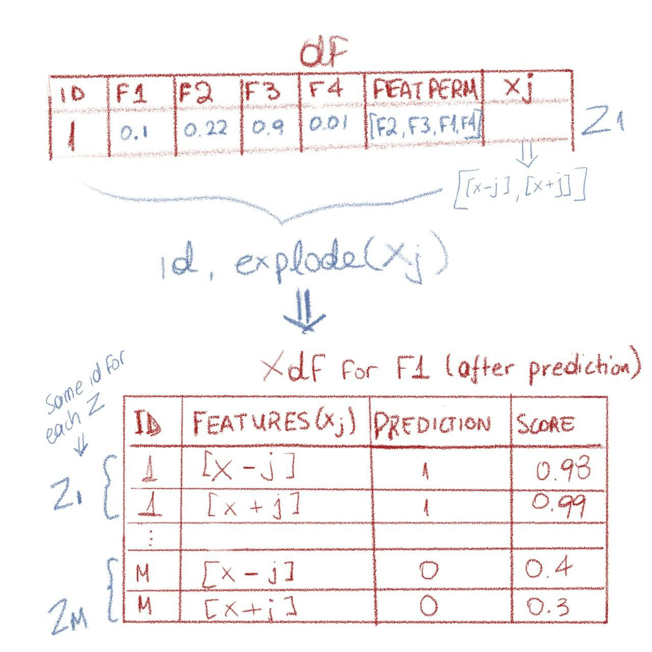 From the dataframe df with xj colum to the exploded Xdf (source: Author)
And next we calculate each z marginal contribution:
*# marginal contribution is calculated using a window and a lag of 1.
# the window is partitioned by id because x+j and x-j for the same row
# will have the same id
*x_df = x_df.withColumn(
    **'marginal_contribution'**,
    (
            F.col(column_to_examine) - F.lag(
                F.col(column_to_examine), 1
            ).over(Window.partitionBy(**'id'**).orderBy(**'id'**)
    )
    )
)
+----+-------------------------------------++-------------+---------------------+
|id  |features                             |prediction    |marginal_contribution|
+----+-------------------------------------+--------------+---------------------+
|1677|[0.349,0.141,0.162,0.162,0.162,0.349]|0.0           |null                 |
|1677|[0.886,0.141,0.162,0.162,0.162,0.349]|0.0           |0.0                  |
|2250|[0.106,0.423,0.777,0.777,0.777,0.886]|0.0           |null                 |
|2250|[0.886,0.423,0.777,0.777,0.777,0.886]|0.0           |0.0                  |
|2453|[0.801,0.423,0.777,0.777,0.87,0.886] |0.0           |null                 |
+----+-------------------------------------+--------------+---------------------+
only showing top 5 rows
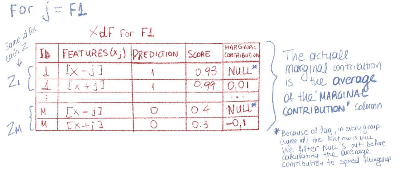 Marginal Contribution calculation (source: Author)
The complete code
import os
from psutil import virtual_memory
from pyspark import SparkConf
from pyspark.ml.linalg import Vectors, VectorUDT
from pyspark.sql import functions as F, SparkSession, types as T, Window


def get_spark_session():
    """
    With an effort to optimize memory and partitions
    """
    mem = virtual_memory()
    conf = SparkConf()
    memory = f'{int(round((mem.total / 2) / 1024 / 1024 / 1024, 0))}G'
    print(memory)
    conf.set('spark.driver.memory', memory)
    conf.set('spark.sql.shuffle.partitions', str(os.cpu_count()*2))
    return SparkSession \
        .builder \
        .config(conf=conf) \
        .appName("IForest feature importance") \
        .getOrCreate()


def get_features_permutations(
        df,
        feature_names,
        output_col='features_permutations'
):
    """
    Creates a column for the ordered features and then shuffles it.
    The result is a dataframe with a column `output_col` that contains:
    [feat2, feat4, feat3, feat1],
    [feat3, feat4, feat2, feat1],
    [feat1, feat2, feat4, feat3],
    ...
    """
    return df.withColumn(
        output_col,
        F.shuffle(
            F.array(*[F.lit(f) for f in feature_names])
        )
    )


def calculate_shapley_values(
        df,
        model,
        row_of_interest,
        feature_names,
        features_col='features',
        column_to_examine='anomalyScore'
):
    """
    # Based on the algorithm described here:
    # https://christophm.github.io/interpretable-ml-book/shapley.html#estimating-the-shapley-value
    # And on Baskerville's implementation for IForest/ AnomalyModel here:
    # https://github.com/equalitie/baskerville/blob/develop/src/baskerville/util/model_interpretation/helpers.py#L235
    """
    results = {}
    features_perm_col = 'features_permutations'
    spark = get_spark_session()
    marginal_contribution_filter = F.avg('marginal_contribution').alias(
        'shap_value'
    )
    # broadcast the row of interest and ordered feature names
    ROW_OF_INTEREST_BROADCAST = spark.sparkContext.broadcast(row_of_interest)
    ORDERED_FEATURE_NAMES = spark.sparkContext.broadcast(feature_names)

    # persist before continuing with calculations
    if not df.is_cached:
        df = df.persist()

    # get permutations
    features_df = get_features_permutations(
        df,
        feature_names,
        output_col=features_perm_col
    )

    # set up the udf - x-j and x+j need to be calculated for every row
    def calculate_x(
            feature_j, z_features, curr_feature_perm
    ):
        """
        The instance  x+j is the instance of interest,
        but all values in the order before feature j are
        replaced by feature values from the sample z
        The instance  x−j is the same as  x+j, but in addition
        has feature j replaced by the value for feature j from the sample z
        """
        x_interest = ROW_OF_INTEREST_BROADCAST.value
        ordered_features = ORDERED_FEATURE_NAMES.value
        x_minus_j = list(z_features).copy()
        x_plus_j = list(z_features).copy()
        f_i = curr_feature_perm.index(feature_j)
        after_j = False
        for f in curr_feature_perm[f_i:]:
            # replace z feature values with x of interest feature values
            # iterate features in current permutation until one before j
            # x-j = [z1, z2, ... zj-1, xj, xj+1, ..., xN]
            # we already have zs because we go row by row with the udf,
            # so replace z_features with x of interest
            f_index = ordered_features.index(f)
            new_value = x_interest[f_index]
            x_plus_j[f_index] = new_value
            if after_j:
                x_minus_j[f_index] = new_value
            after_j = True

        # minus must be first because of lag
        return Vectors.dense(x_minus_j), Vectors.dense(x_plus_j)

    udf_calculate_x = F.udf(calculate_x, T.ArrayType(VectorUDT()))

    # persist before processing
    features_df = features_df.persist()

    for f in feature_names:
        # x column contains x-j and x+j in this order.
        # Because lag is calculated this way:
        # F.col('anomalyScore') - (F.col('anomalyScore') one row before)
        # x-j needs to be first in `x` column array so we should have:
        # id1, [x-j row i,  x+j row i]
        # ...
        # that with explode becomes:
        # id1, x-j row i
        # id1, x+j row i
        # ...
        # to give us (x+j - x-j) when we calculate marginal contribution
        # Note that with explode, x-j and x+j for the same row have the same id
        # This gives us the opportunity to use lag with
        # a window partitioned by id
        x_df = features_df.withColumn('x', udf_calculate_x(
            F.lit(f), features_col, features_perm_col
        )).persist()
        print(f'Calculating SHAP values for "{f}"...')

        x_df = x_df.selectExpr(
            'id', f'explode(x) as {features_col}'
        ).cache()
        x_df = model.transform(x_df)

        # marginal contribution is calculated using a window and a lag of 1.
        # the window is partitioned by id because x+j and x-j for the same row
        # will have the same id
        x_df = x_df.withColumn(
            'marginal_contribution',
            (
                    F.col(column_to_examine) - F.lag(
                        F.col(column_to_examine), 1
                    ).over(Window.partitionBy('id').orderBy('id')
            )
            )
        )
        # calculate the average
        x_df = x_df.filter(
            x_df.marginal_contribution.isNotNull()
        )
        results[f] = x_df.select(
            marginal_contribution_filter
        ).first().shap_value
        x_df.unpersist()
        del x_df
        print(f'Marginal Contribution for feature: {f} = {results[f]} ')

    ordered_results = sorted(
        results.items(),
        key=operator.itemgetter(1),
        reverse=True
    )
    return ordered_results
How to use it
The following code generates a random dataset of 6 features, F1, F2, F3, F4, F5, F6 , with labels [0, 1] and uses the shapley_spark_calculation above to figure out which features seem to work best for a random row of interest. Then it uses only the top 3 features and calculates accuracy again to see whether it is improved. After that it uses the last 3 features in the feature ranking, presumably those who perform worse, to see whether this is indeed true.
This is a very naive and simple example and since the dataframe consists of random values, the accuracy and test error are around 0.5 — coin toss probability. Which also means that different runs yield different results and while most of the times it works as expected and the Shapley feature ranking indeed provides better results, this is not always the case. This is just for demonstrative reasons on how to use the calculate_shapley_values function. Also note that it currently uses the prediction column, but for IForest, it would be more beneficial to use the `anomalyScore` column.
Final output sample on the random dataset:
Feature ranking by Shapley values:
--------------------
#0. f4 = 0.0020181634712411706
#1. f3 = 0.0010090817356205853
#2. f1 = 0.0
#3. f2 = -0.0010090817356205853
#4. f0 = -0.006054490413723511
#5. f5 = -0.007063572149344097
*To be implemented: use rawPrediction or probabilities to evaluate models.*
import random

import numpy as np
import pyspark
from shapley_spark_calculation import \
    calculate_shapley_values, select_row
from pyspark.ml.classification import RandomForestClassifier, LinearSVC, \
    DecisionTreeClassifier
from pyspark.ml.evaluation import BinaryClassificationEvaluator
from pyspark.ml.feature import VectorAssembler
from pyspark.sql import SparkSession, types as T, functions as F


def get_spark_session():
    import os
    from psutil import virtual_memory
    from pyspark import SparkConf

    mem = virtual_memory()
    conf = SparkConf()
    memory = f'{int(round((mem.total / 2) / 1024 / 1024 / 1024, 0))}G'
    print(memory)
    conf.set('spark.driver.memory', memory)
    conf.set('spark.sql.shuffle.partitions', str(os.cpu_count()*2))
    return SparkSession \
        .builder \
        .config(conf=conf) \
        .appName("IForest feature importance") \
        .getOrCreate()


def get_features_schema(feature_names):
    return T.StructType([
        T.StructField(
            name=feature,
            dataType=T.FloatType(),
            nullable=True) for feature in feature_names
    ])


def generate_df_for_features(feature_names, rows=5000):
    data = np.zeros([rows, len(feature_names)])
    spark = get_spark_session()
    df = spark.createDataFrame(
        data.tolist(),
        schema=get_features_schema(feature_names)
    )
    df = df.rdd.zipWithIndex().toDF()
    df = df.withColumnRenamed('_2', 'id')
    for feat in feature_names:
        df = df.withColumn(feat, F.col(f'_1.{feat}')).withColumn(
            feat, F.round(F.rand(random.randint(0, 10)), 3)
        )
    df = df.drop('_1')
    df.show(10, False)
    return df


def add_labels(df: pyspark.sql.DataFrame, labels=(0, 1), split=(.8, .2)):
    if len(labels) > 2:
        raise NotImplementedError
    df_first_label = df.sample(
        fraction=split[0], seed=42
    ).withColumn('label', F.lit(labels[0]))

    return df.join(
        df_first_label.select('id', 'label').alias('df_first_label'),
        on=['id'],
        how='left'
    ).fillna(labels[1], subset=['label'])


if __name__ == '__main__':
    feature_names = [f'f{i}' for i in range(6)]
    spark = get_spark_session()
    df = generate_df_for_features(feature_names, 5000)
    assembler = VectorAssembler(
        inputCols=feature_names,
        outputCol="features")
    df = assembler.transform(df)
    df.show(10, False)
    df = add_labels(df)
    (trainingData, testData) = df.randomSplit([0.8, 0.2])

    estimator = DecisionTreeClassifier(
        labelCol="label", featuresCol="features",
    )
    # estimator = RandomForestClassifier(
    #     labelCol="label", featuresCol="features", numTrees=10
    # )
    model = estimator.fit(trainingData)
    predictions = model.transform(testData)
    column_to_examine = 'prediction'
    predictions.select(column_to_examine, "label", "features").show(5)

    evaluator = BinaryClassificationEvaluator(
        labelCol="label", rawPredictionCol=column_to_examine
    )
    accuracy = evaluator.evaluate(predictions)
    print(f'Test Error = %{(1.0 - accuracy)}')

    testData = select_row(testData, testData.select('id').take(1)[0].id)
    row_of_interest = testData.select('id', 'features').where(
        F.col('is_selected') == True  # noqa
    ).first()
    print('Row: ', row_of_interest)
    testData = testData.select('*').where(F.col('is_selected') != True)
    df = df.drop(
        column_to_examine
    )
    shap_values = calculate_shapley_values(
        testData,
        model,
        row_of_interest,
        feature_names,
        features_col='features',
        column_to_examine='prediction',
    )
    print('Feature ranking by Shapley values:')
    print('-' * 20)


    top_three = []
    last_three = []
    for i, (feat, value) in enumerate(shap_values):
        print(f'#{i}. {feat} = {value}')
        if i < 3:
            top_three.append(feat)
        if i >= 3:
            last_three.append(feat)
    # re-test wiht top 3 features
    trainingData_top_3 = trainingData.select('id', *top_three, 'label')
    testData_top_3= trainingData.select('id', *top_three, 'label')
    assembler_new = VectorAssembler(
        inputCols=top_three,
        outputCol="features")
    trainingData_top_3 = assembler_new.transform(trainingData_top_3)
    testData_top_3 = assembler_new.transform(testData_top_3)
    model = estimator.fit(trainingData_top_3)
    predictions_top_3 = model.transform(testData_top_3)
    accuracy_top_3 = evaluator.evaluate(predictions_top_3)
    print(f'Test Error = %{(1.0 - accuracy_top_3)}')

    print('Top3: Improved by', accuracy_top_3 - accuracy)
    assert accuracy_top_3 > accuracy

    # re-test wiht last 3 features
    trainingData_last_3 = trainingData.select('id', *last_three, 'label')
    testData_last_3 = trainingData.select('id', *last_three, 'label')
    assembler_new = VectorAssembler(
        inputCols=last_three,
        outputCol="features")
    trainingData_last_3 = assembler_new.transform(trainingData_last_3)
    testData_last_3 = assembler_new.transform(testData_last_3)
    model = estimator.fit(trainingData_last_3)
    predictions_last_3 = model.transform(testData_last_3)
    accuracy_last_3 = evaluator.evaluate(predictions_last_3)
    print(f'Test Error = %{(1.0 - accuracy_last_3)}')

    print('Last 3: Worse by', accuracy_last_3 - accuracy_top_3)
    assert accuracy_last_3 < accuracy_top_3
CLI
import operator
import os

import time
import warnings

from pyspark.ml.linalg import Vectors, VectorUDT
from pyspark.sql import functions as F, SparkSession, types as T, Window


def class_from_str(str_class):
    """
    Imports the module that contains the class requested and returns
    the class
    :param str_class: the full path to class, e.g. pyspark.sql.DataFrame
    :return: the class requested
    """
    import importlib

    split_str = str_class.split('.')
    class_name = split_str[-1]
    module_name = '.'.join(split_str[:-1])
    module = importlib.import_module(module_name)

    return getattr(module, class_name)


def get_model_metadata(model_path):
    """
    Loads model metadata from saved model path
    """
    import json
    with open(os.path.join(model_path, 'metadata', 'part-00000')) as mp:
        return json.load(mp)


def load_model(model_path, metadata):
    """
    Returns the model instance based on the metadata class. It is assumed that
    the spark session has been instantiated with the proper spark.jars
    """
    return class_from_str(
        metadata['class']
    ).load(model_path)


def load_df_with_expanded_features(
        df_path, feature_names, features_col='features'
):
    spark = get_spark_session()
    df = spark.read.json(df_path).cache()
    if features_col in df.columns:
        df = expand_features(df, feature_names, features_col)
    return df


def load_df_from_json(df_path):
    """
    Load the spark dataframe - json format
    """
    return get_spark_session().read.json(df_path).cache()


def expand_features(df, feature_names, features_col='features'):
    """
    Return a dataframe with as many extra columns as the feature_names
    """
    for feature in feature_names:
        column = f'{features_col}.{feature}'
        df = df.withColumn(
            column, F.col(column).cast('double').alias(feature)
        )
    return df


def get_spark_session():
    import os
    from psutil import virtual_memory
    from pyspark import SparkConf

    mem = virtual_memory()
    conf = SparkConf()
    memory = f'{int(round((mem.total / 2) / 1024 / 1024 / 1024, 0))}G'
    print(memory)
    conf.set('spark.driver.memory', memory)
    conf.set('spark.sql.shuffle.partitions', str(os.cpu_count()*2))
    return SparkSession \
        .builder \
        .config(conf=conf) \
        .appName("IForest feature importance") \
        .getOrCreate()


def select_row(df, row_id):
    """
    Mark row as selected
    """
    return df.withColumn(
        'is_selected',
        F.when(F.col('id') == row_id, F.lit(True)).otherwise(F.lit(False))
    )


def get_features_permutations(
        df,
        feature_names,
        output_col='features_permutations'
):
    """
    Creates a column for the ordered features and then shuffles it.
    The result is a dataframe with a column `output_col` that contains:
    [feat2, feat4, feat3, feat1],
    [feat3, feat4, feat2, feat1],
    [feat1, feat2, feat4, feat3],
    ...
    """
    return df.withColumn(
        output_col,
        F.shuffle(
            F.array(*[F.lit(f) for f in feature_names])
        )
    )


def calculate_shapley_values(
        df,
        model,
        row_of_interest,
        feature_names,
        features_col='features',
        column_to_examine='anomalyScore'
):
    """
    # Based on the algorithm described here:
    # https://christophm.github.io/interpretable-ml-book/shapley.html#estimating-the-shapley-value
    # And on Baskerville's implementation for IForest/ AnomalyModel here:
    # https://github.com/equalitie/baskerville/blob/develop/src/baskerville/util/model_interpretation/helpers.py#L235
    """
    results = {}
    features_perm_col = 'features_permutations'
    spark = get_spark_session()
    marginal_contribution_filter = F.avg('marginal_contribution').alias(
        'shap_value'
    )
    # broadcast the row of interest and ordered feature names
    ROW_OF_INTEREST_BROADCAST = spark.sparkContext.broadcast(
        row_of_interest[features_col]
    )
    ORDERED_FEATURE_NAMES = spark.sparkContext.broadcast(feature_names)

    # persist before continuing with calculations
    if not df.is_cached:
        df = df.persist()

    # get permutations
    features_df = get_features_permutations(
        df,
        feature_names,
        output_col=features_perm_col
    )

    # set up the udf - x-j and x+j need to be calculated for every row
    def calculate_x(
            feature_j, z_features, curr_feature_perm
    ):
        """
        The instance  x+j is the instance of interest,
        but all values in the order before feature j are
        replaced by feature values from the sample z
        The instance  x−j is the same as  x+j, but in addition
        has feature j replaced by the value for feature j from the sample z
        """
        x_interest = ROW_OF_INTEREST_BROADCAST.value
        ordered_features = ORDERED_FEATURE_NAMES.value
        x_minus_j = list(z_features).copy()
        x_plus_j = list(z_features).copy()
        f_i = curr_feature_perm.index(feature_j)
        after_j = False
        for f in curr_feature_perm[f_i:]:
            # replace z feature values with x of interest feature values
            # iterate features in current permutation until one before j
            # x-j = [z1, z2, ... zj-1, xj, xj+1, ..., xN]
            # we already have zs because we go row by row with the udf,
            # so replace z_features with x of interest
            f_index = ordered_features.index(f)
            new_value = x_interest[f_index]
            x_plus_j[f_index] = new_value
            if after_j:
                x_minus_j[f_index] = new_value
            after_j = True

        # minus must be first because of lag
        return Vectors.dense(x_minus_j), Vectors.dense(x_plus_j)

    udf_calculate_x = F.udf(calculate_x, T.ArrayType(VectorUDT()))

    # persist before processing
    features_df = features_df.persist()

    for f in feature_names:
        # x column contains x-j and x+j in this order.
        # Because lag is calculated this way:
        # F.col('anomalyScore') - (F.col('anomalyScore') one row before)
        # x-j needs to be first in `x` column array so we should have:
        # id1, [x-j row i,  x+j row i]
        # ...
        # that with explode becomes:
        # id1, x-j row i
        # id1, x+j row i
        # ...
        # to give us (x+j - x-j) when we calculate marginal contribution
        # Note that with explode, x-j and x+j for the same row have the same id
        # This gives us the opportunity to use lag with
        # a window partitioned by id
        x_df = features_df.withColumn('x', udf_calculate_x(
            F.lit(f), features_col, features_perm_col
        )).persist()
        print(f'Calculating SHAP values for "{f}"...')
        x_df.show(10, False)
        x_df = x_df.selectExpr(
            'id', f'explode(x) as {features_col}'
        ).cache()
        print('Exploded df:')
        x_df.show(10, False)
        x_df = model.transform(x_df)

        # marginal contribution is calculated using a window and a lag of 1.
        # the window is partitioned by id because x+j and x-j for the same row
        # will have the same id
        x_df = x_df.withColumn(
            'marginal_contribution',
            (
                    F.col(column_to_examine) - F.lag(
                        F.col(column_to_examine), 1
                    ).over(Window.partitionBy('id').orderBy('id')
            )
            )
        )
        x_df.show(5, False)
        # calculate the average
        x_df = x_df.filter(
            x_df.marginal_contribution.isNotNull()
        )
        tdf = x_df.select(
            marginal_contribution_filter
        )
        tdf.show()
        results[f] = x_df.select(
            marginal_contribution_filter
        ).first().shap_value
        x_df.unpersist()
        del x_df
        print(f'Marginal Contribution for feature: {f} = {results[f]} ')

    ordered_results = sorted(
        results.items(),
        key=operator.itemgetter(1),
        reverse=True
    )
    return ordered_results


def shapley_values_for_model(
        model_path,
        feature_names,
        row_id,
        data_path=None,
        column_to_examine=None
):
    from baskerville.spark import get_spark_session
    _ = get_spark_session()
    metadata = get_model_metadata(model_path)
    model = load_model(model_path, metadata)
    features_col = metadata['paramMap'].get('featuresCol', 'features')
    # get sample dataset
    df = load_df_from_json(data_path)
    if 'id' not in df.columns:
        # not a good idea
        warnings.warn('Missing column "id", using monotonically_increasing_id')
        df = df.withColumn('id', F.monotonically_increasing_id())
    df.show(10, False)

    # predict on the data if the df does not contain the results
    if column_to_examine not in df.columns:
        pred_df = model.predict(df)
        df = pred_df.select('id', features_col, column_to_examine)

    # select the row to be examined
    df = select_row(df, row_id)
    row_of_interest = df.select('id', 'features').where(
        F.col('is_selected') == True  # noqa
    ).first()
    print('Row: ', row_of_interest)

    # remove x and drop column_to_examine column
    df = df.select('*').where(
        F.col('is_selected') == False  # noqa
    ).drop(column_to_examine)

    shap_values = calculate_shapley_values(
        df,
        model,
        row_of_interest,
        feature_names,
        features_col=features_col,
        column_to_examine=column_to_examine,
    )
    print('Feature ranking by Shapley values:')
    print('-' * 20)
    print(*[f'#{i}. {feat} = {value}' for i, (feat, value) in
            enumerate(shap_values)])
    return shap_values


if __name__ == '__main__':
    import argparse

    parser = argparse.ArgumentParser()
    parser.add_argument(
        'modelpath', help='The path to the model to be examined'
    )
    parser.add_argument(
        'feature_names',
        help='The feature names. E.g. feature1,feature2,feature3',
        nargs='+', default=[]
    )

    parser.add_argument(
        'datapath', help='The path to the data'
    )
    parser.add_argument(
        'id',
        help='The row id to be examined',
        type=str
    )
    parser.add_argument(
        '-c', '--column',
        help='Column to examine, e.g. prediction. '
             'Default is "anomalyScore"',
        default='anomalyScore',
        type=str
    )
    args = parser.parse_args()
    model_path = args.modelpath
    feature_names = args.feature_names
    data_path = args.datapath
    column_to_examine = args.column
    row_id = args.id

    if not os.path.isdir(model_path):
        raise ValueError('Model path does not exist')
    if not os.path.isdir(data_path):
        raise ValueError('Data path does not exist')

    start = time.time()
    print('Start:', start)
    shapley_values_for_model(
        model_path,
        feature_names,
        row_id,
        data_path,
        column_to_examine
    )
    end = time.time()
    print('End:', end)
    print(f'Calculation took {int(end - start)} seconds')
Disclaimer: This work was based upon opensource work done for the Baskerville project for eQualitie as a Lead Developer on the project — an article for Baskerville will follow :). The Baskerville code was expanded to work for any pyspark model for the article’s purposes. You can find the Baskerville implementation here: equalitie/baskerville Security Analytics Engine — Anomaly Detection in Web Traffic — equalitie/baskervillegithub.com equalitie/baskerville Security Analytics Engine — Anomaly Detection in Web Traffic — equalitie/baskervillegithub.com
Useful links
The python shap package has some very interesting examples in their docs: An introduction to explainable AI with Shapley values — SHAP latest documentation The gray horizontal line in the plot above represents the expected value of the model when applied to the boston…shap.readthedocs.io slundberg/shap SHAP (SHapley Additive exPlanations) is a game theoretic approach to explain the output of any machine learning model…github.com
Examples of how to use the python shap library can be found here: SHAP Values Explore and run machine learning code with Kaggle Notebooks | Using data from multiple data sourceskaggle.com
The python shap library also has very beautiful visualizations. Isolation Forest and Spark Main characteristics and ways to use Isolation Forest in PySparktowardsdatascience.com
Notes
Part of the reason for writing this article here is to get a review of the process, in case I missed anything. So, please, feel free to send me your comments and thoughts about this. I’d love to know if there’s any better way of implementing the Shapley values calculation and if there is already something out there that does a better job.
Another reason is that we, in Baskerville, have tested this in production and it has helped us a lot with having better results. You can see Baskerville’s performance stats here:
https://deflect.ca/solutions/deflect-labs/baskerville/
Thanks and take care!