

Main characteristics and ways to use Isolation Forest in PySpark
Isolation Forest is an algorithm for anomaly / outlier detection, basically a way to spot the odd one out. We go through the main characteristics and explore two ways to use Isolation Forest with Pyspark.
Isolation Forest for Outlier Detection
Most existing model-based approaches to anomaly detection construct a profile of normal instances, then identify instances that do not conform to the normal profile as anomalies. […] [Isolation Forest] explicitly isolates anomalies instead of profiles normal points
source: https://cs.nju.edu.cn/zhouzh/zhouzh.files/publication/icdm08b.pdf
Isolation means separating an instance from the rest of the instances
Basic Characteristics of Isolation Forest
it uses normal samples as the training set and can allow a few instances of abnormal samples (configurable). You basically feed the algorithm your normal data and it doesn’t mind if your dataset is not that well curated, provided you tune the
contaminationparameter. In other words it learns what normal looks like to be able to distinguish the abnormal,it works with the basic assumption that anomalies are few and easily distinguishable,
it has a linear time complexity with a low constant and a low memory requirements*,
it is fast because it doesn’t utilize any distance or density measures,
can scale up very well. It seems to work well with high dimensional problems that may have a large number of irrelevant attributes.
*low memory requirements come from the fact that each tree in the forest does not have to be constructed the wholly, since the anomalies should have a lot shorter paths than the normal instances, so a max depth can be used to cut off the tree construction.
Isolation Forest takes advantage of the two characteristics of anomalies: that they are few and distinct / different
Anomaly Score and Path Length
One way to detect anomalies is to sort data points according to their path lengths or anomaly scores; and anomalies are points that are ranked at the top of the list
Path length: the number of edges until we reach an external node
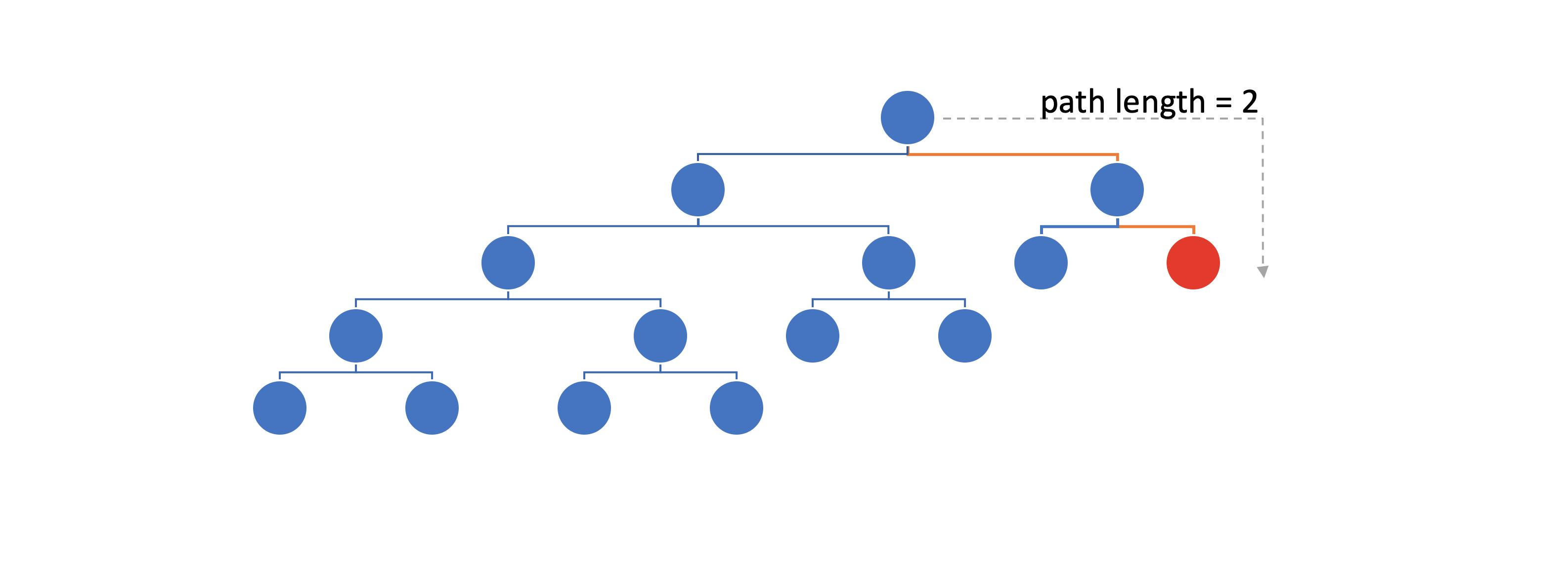 Example of a path length calculation
Anomaly Score
This is basically the output of the algorithm, which is ≤1 and ≥0. This is where the path length come in the picture. With the estimation of the average path length in the whole forest, we can deduce whether a point is anomalous or not.
If the anomaly score for an instance is very close to 1 then it is safe to say that this instance is an anomaly, if it is < 0.5 then it is probably a normal instance and if it is ~= 0.5 then the entire sample does not have any distinct anomalies.
Important parameters in Isolation Forest
number of trees / estimators : how big is the forest
contamination: the fraction of the dataset that contains abnormal instances, e.g. 0.1 or 10%
max samples: The number of samples to draw from the training set to train each Isolation Tree with.
max depth: how deep the tree should be, this can be used to trim the tree and make things faster.
The algorithm learns what normal looks like to be able to distinguish the abnormal
How to use it with PySpark
The Scikit-learn Way
The Scikit-learn way will need us to create a udf to be able to predict upon a dataframe. This is the usual way in general to utilize a Scikit-learn model. Note that we cannot parallelize the training part using spark — but we can use the parameter n_jobs=-1 to utilize all cores on our machine. Another important thing to remember is to set the random_seed to something specific so that the results are reproducible.
All we need to do is install scikit-learn and its dependenciespip install sklearn numpy scipy
Then we can start with a simple example, a dataframe with four samples.
from pyspark.sql import SparkSession, functions as F, types as T
from sklearn.ensemble import IsolationForest
from sklearn.preprocessing import StandardScaler

np.random.seed(42)

conf = SparkConf()
spark_session = SparkSession.builder \
    .config(conf=conf) \
    .appName('test') \
    .getOrCreate()

# create a dataframe
data = [
    {'feature1': 1., 'feature2': 0., 'feature3': 0.3, 'feature4': 0.01},
    {'feature1': 10., 'feature2': 3., 'feature3': 0.9, 'feature4': 0.1},
    {'feature1': 101., 'feature2': 13., 'feature3': 0.9, 'feature4': 0.91},
    {'feature1': 111., 'feature2': 11., 'feature3': 1.2, 'feature4': 1.91},
]
df = spark_session.createDataFrame(data)
df.show()

# instantiate a scaler, an isolation forest classifier and convert the data into the appropriate form
scaler = StandardScaler()
classifier = IsolationForest(contamination=0.3, random_state=42, n_jobs=-1)
x_train = [list(n.values()) for n in data]

# fit on the data
x_train = scaler.fit_transform(x_train)
clf = classifier.fit(x_train)

# broadcast the scaler and the classifier objects
# remember: broadcasts work well for relatively small objects
SCL = spark_session.sparkContext.broadcast(scaler)
CLF = spark_session.sparkContext.broadcast(clf)


def predict_using_broadcasts(feature1, feature2, feature3, feature4):
    """
    Scale the feature values and use the model to predict
    :return: 1 if normal, -1 if abnormal 0 if something went wrong
    """
    prediction = 0

    x_test = [[feature1, feature2, feature3, feature4]]
    try:
        x_test = SCL.value.transform(x_test)
        prediction = CLF.value.predict(x_test)[0]
    except ValueError:
        import traceback
        traceback.print_exc()
        print('Cannot predict:', x_test)

    return int(prediction)


udf_predict_using_broadcasts = F.udf(predict_using_broadcasts, T.IntegerType())


df = df.withColumn(
    'prediction',
    udf_predict_using_broadcasts('feature1', 'feature2', 'feature3', 'feature4')
)

df.show()

+--------+--------+--------+--------+
|feature1|feature2|feature3|feature4|
+--------+--------+--------+--------+
|     1.0|     0.0|     0.3|    0.01|
|    10.0|     3.0|     0.9|     0.1|
|   101.0|    13.0|     0.9|    0.91|
|   111.0|    11.0|     1.2|    1.91|
+--------+--------+--------+--------+

+--------+--------+--------+--------+----------+
|feature1|feature2|feature3|feature4|prediction|
+--------+--------+--------+--------+----------+
|     1.0|     0.0|     0.3|    0.01|        -1|
|    10.0|     3.0|     0.9|     0.1|         1|
|   101.0|    13.0|     0.9|    0.91|         1|
|   111.0|    11.0|     1.2|    1.91|         1|
+--------+--------+--------+--------+----------+
There is more than one way to go about this udf, for example you can load the model within the udf from a file (which can potentially cause errors because of the parallelization), or you could pass the serialized model as a column (which will increase your memory consumption by a lot), but I’ve found that the use of broadcast variables works best in terms of time and memory performance.
Let me know if there’s a better way to do this :)
The Spark-ML way
There is no official package for iForest in the Spark ML library currently. However, I’ve found two implementations, one by LinkedIn which only has the Scala implementation and one by Fangzhou Yang that can be used with Spark and PySpark. We’ll explore the second one.
Steps to use spark-iforest by Fangzhou Yang:
Clone the repository
Build the jar (you’ll need Maven for this)
cd spark-iforest/

mvn clean package -DskipTests
- And either copy it to
$SPARK_HOME/jars/or provide it as extra jar in your spark configuration (I prefer the latter for more flexibility):
cp target/spark-iforest-<version>.jar $SPARK_HOME/jars/
or
conf = SparkConf()
conf.set('spark.jars', '/full/path/to/target/spark-iforest-<version>.jar')

spark_session = SparkSession.builder.config(conf=conf).appName('IForest').getOrCreate()
- Install the python version of spark-iforest:
cd spark-iforest/python

pip install -e .   # skip the -e flag if you don't want to edit the project
And we’re ready to use it! Again, it is important to set the random seed to something specific for reproducibility.
from pyspark import SparkConf
from pyspark.sql import SparkSession, functions as F
from pyspark.ml.feature import VectorAssembler, StandardScaler
from pyspark_iforest.ml.iforest import IForest, IForestModel
import tempfile

conf = SparkConf()
conf.set('spark.jars', '/full/path/to/spark-iforest/target/spark-iforest-2.4.0.jar')

spark = SparkSession \
        .builder \
        .config(conf=conf) \
        .appName("IForestExample") \
        .getOrCreate()

temp_path = tempfile.mkdtemp()
iforest_path = temp_path + "/iforest"
model_path = temp_path + "/iforest_model"

# same data as in https://gist.github.com/mkaranasou/7aa1f3a28258330679dcab4277c42419
# for comparison
data = [
    {'feature1': 1., 'feature2': 0., 'feature3': 0.3, 'feature4': 0.01},
    {'feature1': 10., 'feature2': 3., 'feature3': 0.9, 'feature4': 0.1},
    {'feature1': 101., 'feature2': 13., 'feature3': 0.9, 'feature4': 0.91},
    {'feature1': 111., 'feature2': 11., 'feature3': 1.2, 'feature4': 1.91},
]

# use a VectorAssembler to gather the features as Vectors (dense)
assembler = VectorAssembler(
    inputCols=list(data[0].keys()),
    outputCol="features"
)

df = spark.createDataFrame(data)
df = assembler.transform(df)
df.show()


# use a StandardScaler to scale the features (as also done in https://gist.github.com/mkaranasou/7aa1f3a28258330679dcab4277c42419)
scaler = StandardScaler(inputCol='features', outputCol='scaledFeatures')
iforest = IForest(contamination=0.3, maxDepth=2)
iforest.setSeed(42)  # for reproducibility

scaler_model = scaler.fit(df)
df = scaler_model.transform(df)
df = df.withColumn('features', F.col('scaledFeatures')).drop('scaledFeatures')
model = iforest.fit(df)

# Check if the model has summary or not, the newly trained model has the summary info
print(model.hasSummary)

# Show the number of anomalies
summary = model.summary
print(summary.numAnomalies)

# Predict for a new data frame based on the fitted model
transformed = model.transform(df)

# Save the iforest estimator into the path
iforest.save(iforest_path)

# Load iforest estimator from a path
loaded_iforest = IForest.load(iforest_path)

# Save the fitted model into the model path
model.save(model_path)

# Load a fitted model from a model path
loaded_model = IForestModel.load(model_path)

# The loaded model has no summary info
print(loaded_model.hasSummary)

# Use the loaded model to predict a new data frame
loaded_model.transform(df).show()

+--------+--------+--------+--------+--------------------+
|feature1|feature2|feature3|feature4|            features|
+--------+--------+--------+--------+--------------------+
|     1.0|     0.0|     0.3|    0.01|  [1.0,0.0,0.3,0.01]|
|    10.0|     3.0|     0.9|     0.1|  [10.0,3.0,0.9,0.1]|
|   101.0|    13.0|     0.9|    0.91|[101.0,13.0,0.9,0...|
|   111.0|    11.0|     1.2|    1.91|[111.0,11.0,1.2,1...|
+--------+--------+--------+--------+--------------------+

True
1
+--------+--------+--------+--------+--------------------+-------------------+----------+
|feature1|feature2|feature3|feature4|            features|       anomalyScore|prediction|
+--------+--------+--------+--------+--------------------+-------------------+----------+
|     1.0|     0.0|     0.3|    0.01|[0.01715764009115...| 0.4947228944353107|       1.0|
|    10.0|     3.0|     0.9|     0.1|[0.17157640091152...| 0.4072150693026707|       0.0|
|   101.0|    13.0|     0.9|    0.91|[1.73292164920643...|0.41181393953312606|       0.0|
|   111.0|    11.0|     1.2|    1.91|[1.90449805011796...| 0.4765458247608175|       0.0|
+--------+--------+--------+--------+--------------------+-------------------+----------+

2019-11-07 16:11:20 WARN  MemoryManager:115 - Total allocation exceeds 95.00% (906,992,014 bytes) of heap memory
Scaling row group sizes to 96.54% for 7 writers
2019-11-07 16:11:20 WARN  MemoryManager:115 - Total allocation exceeds 95.00% (906,992,014 bytes) of heap memory
Scaling row group sizes to 84.47% for 8 writers
[Stage 23:>                                                         (0 + 8) / 8]2019-11-07 16:11:20 WARN  MemoryManager:115 - Total allocation exceeds 95.00% (906,992,014 bytes) of heap memory
Scaling row group sizes to 96.54% for 7 writers
False
+--------+--------+--------+--------+--------------------+-------------------+----------+
|feature1|feature2|feature3|feature4|            features|       anomalyScore|prediction|
+--------+--------+--------+--------+--------------------+-------------------+----------+
|     1.0|     0.0|     0.3|    0.01|[0.01715764009115...| 0.4947228944353107|       1.0|
|    10.0|     3.0|     0.9|     0.1|[0.17157640091152...| 0.4072150693026707|       0.0|
|   101.0|    13.0|     0.9|    0.91|[1.73292164920643...|0.41181393953312606|       0.0|
|   111.0|    11.0|     1.2|    1.91|[1.90449805011796...| 0.4765458247608175|       0.0|
+--------+--------+--------+--------+--------------------+-------------------+----------+
Results
In both examples we use a very small and simple dataset, just to demonstrate the process.
data = [
    {**'feature1'**: 1., **'feature2'**: 0., **'feature3'**: 0.3, **'feature4'**: 0.01},
    {**'feature1'**: 10., **'feature2'**: 3., **'feature3'**: 0.9, **'feature4'**: 0.1},
    {**'feature1'**: 101., **'feature2'**: 13., **'feature3'**: 0.9, **'feature4'**: 0.91},
    {**'feature1'**: 111., **'feature2'**: 11., **'feature3'**: 1.2, **'feature4'**: 1.91},
]
Both implementations of the algorithm conclude that the first sample looks anomalous in comparison to the other three samples, which makes sense if we take a look at the features.
Note the different range of the outputs: [-1, 1] vs [0, 1]
Output of scikit-learn IsolationForest (-1 means anomalous/ outlier, 1 means normal/ inlier)
+--------+--------+--------+--------+----------+
|feature1|feature2|feature3|feature4|prediction|
+--------+--------+--------+--------+----------+
|     1.0|     0.0|     0.3|    0.01|        -1|
|    10.0|     3.0|     0.9|     0.1|         1|
|   101.0|    13.0|     0.9|    0.91|         1|
|   111.0|    11.0|     1.2|    1.91|         1|
+--------+--------+--------+--------+----------+

Output of spark-iforest implementation (1.0 means anomalous/ outlier, 0.0 normal/ inlier):
+--------+--------+--------+--------+----------+
|feature1|feature2|feature3|feature4|prediction|
+--------+--------+--------+--------+----------+
|     1.0|     0.0|     0.3|    0.01|       1.0|
|    10.0|     3.0|     0.9|     0.1|       0.0|
|   101.0|    13.0|     0.9|    0.91|       0.0|
|   111.0|    11.0|     1.2|    1.91|       0.0|
+--------+--------+--------+--------+----------+
Edit:
It seems that IForest can handle currently only DenseVector input, while VectorAssembler outputs both Dense and Sparse vectors. So, unfortunately, we need to convert the vectors to Dense using a udf.
**from **pyspark.ml.linalg **import **Vectors, VectorUDT
**from **pyspark.sql **import **functions **as **F
**from **pyspark.sql **import **types **as **T

list_to_vector_udf = F.udf(lambda l: Vectors.dense(l), VectorUDT())

data.withColumn(
    'vectorized_features',
    list_to_vector_udf('features')
)
...
Conclusion
Isolation Forest, in my opinion, is a very interesting algorithm, light, scalable, with many applications. It is definitely worth exploring.
For the Pyspark integration: I’ve used the Scikit-learn model quite extensively and while it works well, I’ve found that as the model size increases, so does the time it takes to broadcast the model and complete a prediction cycle. As expected.
I haven’t tested the PySpark ML way enough to be certain that both implementations give the same results, but in the small, meaningless dataset I used in the examples, they seem to agree. I will definitely experiment more with this to investigate how well it scales and how good the outcome is.
I hope this was helpful and that knowing about how to use Isolation Forest in combination with PySpark will save you some time and trouble. Any thoughts, questions, corrections and suggestions are very welcome :)
If you want to know more about how Spark works, take a look at: Explaining technical stuff in a non-technical way — Apache Spark What is Spark and PySpark and what can I do with it?towardsdatascience.com Adding sequential IDs to a Spark Dataframe How to do it and is it a good idea?towardsdatascience.com
And if you are coming from the Pandas world and want to get hands on quickly with Spark, check out Koalas: From Pandas to PySpark with Koalas The Koalas project makes data scientists more productive when interacting with big data, by implementing the pandas…towardsdatascience.com
Useful links
Isolation Forest paper: https://cs.nju.edu.cn/zhouzh/zhouzh.files/publication/icdm08b.pdf sklearn.ensemble.IsolationForest - scikit-learn 0.21.3 documentation class sklearn.ensemble. IsolationForest( n_estimators=100, max_samples='auto', contamination='legacy'…scikit-learn.org Isolation Forest Step by Step Overviewmedium.com titicaca/spark-iforest Isolation Forest (iForest) is an effective model that focuses on anomaly isolation. iForest uses tree structure for…github.com linkedin/isolation-forest This is a Scala/Spark implementation of the Isolation Forest unsupervised outlier detection algorithm. This library was…github.com
Next
Understanding Isolation Forest’s predictions using Shapley Values — Estimating feature importance at scale: Machine Learning Interpretability — Shapley Values with PySpark Interpreting Isolation Forest’s predictions — and not onlymedium.com